Quickstart

Install

# install via pip
# requires python 3; tested for python 3.4 and up
pip install pytrails

Example

Let’s assume, we have observed a sequence of rainy and sunny days. To explain what we have observed, we have two hypotheses:

• sticky: when it is sunny it stays sunny, and when it rains it stays rainy
• random: the weather is totally random

We want to test, which one of these hypotheses is more plausible given our observations. To this end we use HypTrails as introduced by Singer et al. in 2015.

In particular, we

• first we calculate transition counts between states
• define hypotheses as transition probability matrices
• calculate the evidence for each hypothesis using a set of increasing concentration factors

import numpy as np
from scipy.sparse import csr_matrix
from pytrails.hyptrails import MarkovChain
import matplotlib.pyplot as plt

# sequence of observations (0 = rainy, 1 = sunny)
observations = [0, 1, 0, 0, 1, 0, 0, 1, 1]

########
# calculate transition counts between states
########
transition_counts = np.zeros((2, 2))
for i in range(len(observations) - 1):
    transition_counts[observations[i], observations[i+1]] += 1
transition_counts = csr_matrix(transition_counts)

########
# define hypotheses as transition probability matrices
########
hyp_sticky = csr_matrix([
    [1.0, 0.0],
    [0.0, 1.0]])

hyp_random = csr_matrix([
    [0.5, 0.5],
    [0.5, 0.5]])

########
# calculate the evidence for each hypothesis using a set of increasing concentration factors:
########

concentration_factors = np.array([0, 1, 2, 3, 4, 5])

# scale concentration factors by number of states
concentration_factors = concentration_factors * transition_counts.shape[0]

# calculate evidences
evidence_sticky = [MarkovChain.marginal_likelihood(transition_counts, hyp_sticky * c) for c in concentration_factors]
evidence_random = [MarkovChain.marginal_likelihood(transition_counts, hyp_random * c) for c in concentration_factors]

########
# plot the results:
########

plt.plot(concentration_factors, evidence_sticky, 'rs--', label="sticky")
plt.plot(concentration_factors, evidence_random, 'bs--', label="random")
plt.legend()
plt.show()

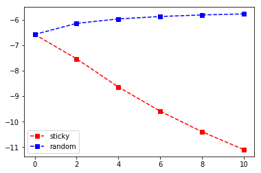
When comparing our results, we see that, our random hypothesis results in higher evidence values (i.e., marginal likelihood). That is, assuming random weather explains our observations better than believing in sticky conditions.